DRCMR Logo 300px Color
 

Quick start guide to the Bloch Simulator

This page provides step-by-step examples to practical use of the Bloch Simulator made for visualizing basic and advanced Magnetic Resonance techniques. The examples are spin-echo formation and the excitation process, which are also demonstrated in corresponding YouTube videos. The basic MR knowledge needed to understand the text below is described in an MRI tutorial targeted at a broad audience.

  • It is easiest to run the simulator directly in an internet browser. If you have not already started it, please do so by following this link starting the software in a new browser window: http://www.drcmr.dk/BlochSimulator
  • If you have Flash installed on your computer, you should now see the magnetization vector of an imaginary sample precessing in a magnetic field, B0, pointing upwards. You can always get back to this situation by choosing "Scene: Precession" in the pull-down menu on the lower left.
  • First try to adjust the B0 field strength by moving the slider named "B0". Notice how the precession frequency changes with the field. Think of the units as tesla, for example.

Spin-echo demonstration, step by step:
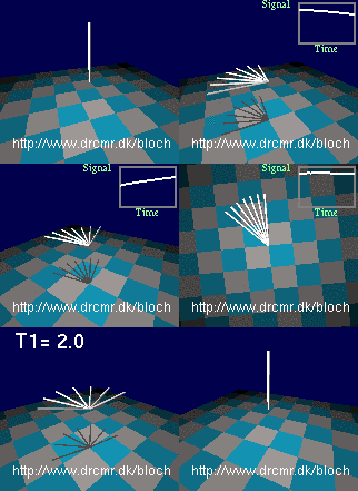
The spin echo sequence
  • Now, let's introduce field inhomogeneity so that all nuclei do not precess at the same frequency. This can be done by choosing "Scene: Weak inhomogeneity" in the pull-down menu on the lower left. You now see the magnetization in thermal equilibrium. The floor rotates since you see this in the rotating frame of resonance which is only needed later. Therefore, shift back to the stationary frame by pressing the  "Change frame"-button.
  • Since weak inhomogeneity was selected above, the nuclei precess at different frequencies, but it does not show until the magnetization is rotated into the transversal plane. Do this by pressing the "90x hard" button (initiates 90 degree RF pulse rotating the magnetization quickly around the x-axis in the transversal plane). You should now see different components of the magnetization precessing at slightly different frequencies. Gradual dephasing leads to a loss of signal seen in the lower right graph. Press the "v" key on keyboard a few times - it toggles the viewing angle.
  • You may want to repeat the last few steps by pressing the "Scene: Weak inhomogeneity" button again and doing a new excitation. Proceed when you understand what you are seeing so far. Let's add a short 180 degree refocusing pulse to our sequence after some dephasing has occurred (press the "180y hard"-button). This will lead to the formation of a spin-echo after a period equal to the dephasing period. Notice how the nuclei get back in phase and how the lost signal is recovered.
  • This finishes the spin-echo demonstration, but you can continue experimenting with it, e.g. by playing out extra refocusing pulses or by adding a bit of relaxation using the T2-slider for example (choose a large value for T2 initially, e.g. 20 seconds). You can also watch the events in the rotating frame of resonance.

Off- and on-resonance excitation, step by step:

  • Go back to the initial situation by  choosing "Scene: Precession" in the pull-down menu on the lower left.
  • Adjust the B0 field strength by moving the slider named "B0". Notice how the precession frequency changes with the field. Set the value of B0 back to 3 by typing the value in the text field above the slider, followed by "enter". Think of the units as tesla, for example.
  • Radio waves applied off-resonance
    Radio waves applied off-resonance
    Now turn on a radio wave field. Do this by setting the RF amplitude to 0.1 using the appropriate slider or by typing the value in the corresponding text field, followed by "enter". The units are the same as for the B0 field. The red bar shows the push of the radio waves on the magnetization (the torque). Notice how the push is orthogonal to the magnetization, and how it rotates.
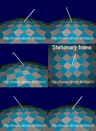
  • The push does not seem to have much of an effect on the magnetization. This is because the frequency of the radio waves is not matched to the Larmor frequency (the radiowaves are off-resonance). The reason for the missing effect may be easier to see in the rotating frame of reference. Press "Change frame" to toggle between viewing in the stationary and the rotating frames of reference as you wish. Notice how the magnetization is not pushed consistently by off-resonance radiowaves (in synchony with the precession). Therefore it just wiggles slightly in the radio wave field. Switch back to the stationary frame of reference.
  • Adjust the radio frequency to match the Larmor frequency simply by setting the RF frequency equal to B0 (3 in this case). This is valid since the gyromagnetic ratio in the simulator is set to 1 Hz/T (approximately). Hence the resonance frequency for a field of value 3 is simply 3. Notice how the magnetization is now gradually changed by the RF field. Watching this in the rotating frame makes it appear much simpler -- switch back and forth a few times, and notice how resonance radiowaves induces rotations in the rotating frame of reference.
  • Radio waves applied on resonance
    Radio waves applied on resonance
    Now you have seen how resonant radiowaves change the magnetization, and how off-resonant waves does not, lets start from equilibrium and do an excitation. Choose "Scene: Equilibrium". Add an RF field by setting the RF amplitude equal to 0.1. Notice how little happens since the RF frequency is not adjusted to the Larmor frequency. Adjust it as described above and see how the magnetization is rotated away from equilibirum, e.g. so it after a while points in the exact opposite directions. Similarly, on-resonance rotations away from equilibrium can be triggered by pressing the buttons labelled "90x hard", "90x selective", "180y hard" and "30x hard" that send bursts of radiowaves sufficiently long to cause the specified rotations.
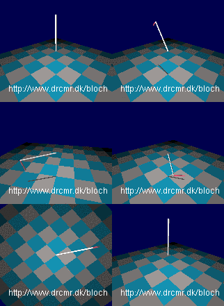

The simulator can do much more. A few examples are given in YouTube videos and on the project homepage but you really need to experiment yourself to get full benefit. The "Challenges" section in the "Help" menu may also be of inspiration.


Selected Publications

Recent publications & Pre-prints 

Naiara Demnitz, Oliver J. Hulme, Hartwig R. Siebner, Michael Kjaer, Klaus P. Ebmeier, Carl-Johan Boraxbekk, Claire M. Gillan (2023). Characterising the covariance pattern between lifestyle factors and structural brain measures: a multivariable replication study of two independent ageing cohorts, Neurobiology of Aging, Volume 131,2023, Pages 115-123, ISSN 0197-4580,IF 3.7.

TH Siebner, JD Hove, CF Madelung, OJ Hulme, F Bendtsen, HR Siebner, Flemming Bendtsen, Mads Barløse (2024). No difference in postprandial mesenteric blood flow between healthy younger and elderly individuals, Scientific Reports 14 (1), 8689.

TS Hjerresen, M Bentz, AB Nejad, E Raffin, KW Andersen, OJ Hulme, Hartwig Roman Siebner, Kerstin Jessica Plessen. Performing well but not appreciating it–A trait feature of anorexia nervosa. JCPP advances 4 (1), e12194.

Oliver Hulme, Arne Vanhoyweghen, Colm Connaughton, Ole Peters, Simon Steinkamp, Alexander Adamou, Dominik Baumann, Vincent Ginis, Bert Verbruggen, James Price, and Benjamin Skjold (2023). Reply to “The Limitations of Growth-Optimal Approaches to Decision Making Under Uncertainty”. Econ Journal Watch, 20(2) p335-348.

Hulme Oliver J., Roulston Barrie, Overgaard Morten (2023). Does report modality modulate psychophysical sensitivity? The jury remains out. Frontiers in Psychology, 14, https://www.frontiersin.org/articles/10.3389/fpsyg.2023.1226588.

Thorup AAE,… Hulme OJ, … Nordentoft M (2022). The Danish High-Risk and Resilience Study-VIA 15 - A Study Protocol for the Third Clinical Assessment of a Cohort of 522 Children Born to Parents Diagnosed With Schizophrenia or Bipolar Disorder and Population-Based Controls. Frontiers in Psychiatry.

Lopez-Yepez JS, Martin J, Hulme OJ, Kvitsiani D. (2021). A normative account of choice history effects in mice and humans. PloS Computational Biology.

Lopez-Yepez JS, Martin J, Hulme OJ, Kvitsiani D. (2021)
A normative account of choice history effects in mice and humans
PLoS Computational Biology

Meder D, Rabe F, Morville T, Madsen KH, Koudahl MT, Dolan RJ, Siebner HR, Hulme OJ. (2021)
Ergodicity-breaking reveals time optimal economic behavior in humans
PLoS Computational Biology

Morville T, Friston KJ, Burdakov D, Siebner HR, Hulme OJ. (Pre-print)
The Homeostatic Logic of Reward
bioRxiv, doi.org/10.1101/242974.

Morville T, Madsen K, Siebner HR, Hulme OJ. (2021)
Reward signaling in brainstem nuclei under glycemic flux
PloS One

Hulme, OJ, Wagenmakers EJ, Damkier P, Madelung CF, Siebner HR, Helweg-Larsen J, Gronau Q, Benfield TL, Madsen KH. (2021) A Bayesian reanalysis of the effects of hydroxychloroquine and azithromycin on viral carriage in patients with COVID-19.
PloS One. doi.org/10.1371/journal.pone.0245048

Friston KJ, Parr T, Zeidman P, Razi A, Flandin G, Daunizau J, Hulme OJ, Billig AJ., Litvak V, Price CJ., Moran RJ., Costello A, Pillay D, Lambert C. (2020)
Effective immunity and second waves: a dynamic causal modelling study
Wellcome Open Res2020, 5:204 (doi.org/10.12688/wellcomeopenres.16253.2)

van der Vegt JPM, Hulme OJ, Madsen KH, Buhmann C, Bloem BR, Münchau A, Helmich RC, Siebner HR (2020)
Dopamine agonist treatment increases sensitivity to gamble outcomes in the hippocampus in de novo Parkinson’s disease
NeuroImage Clinical

Faranda D, Castillo IP, Hulme OJ, Jezequel A, Lamb J, Sato Y, Thompson E, (2020)                                                                         
Asymptotic estimates of SARS-CoV-2 infection counts and their sensitivity to stochastic perturbation
Chaos. 2020;30(5):051107. doi:10.1063/5.0008834

Friston KJ, Parr T, Zeidman P, Razi A, Flandin G, Daunizau J, Hulme OJ, Billig AJ, Litvak V, Price CJ, Moran RJ., Lambert C. (2020)
Second waves, social distancing, and the spread of COVID-19 across America.
Wellcome Open Res 2020, 5:103 (doi.org/10.12688/wellcomeopenres.15986.1)

Friston KJ, Parr T, Zeidman P, Razi A, Flandin G, Daunizau J, Hulme OJ, Billig AJ, Litvak V, Price CJ, Moran RJ, Lambert C. (2020)
Dynamic causal modelling of COVID-19.
Wellcome Open Res 2020, 5:89

Friston KJ, Parr T, Zeidman P, Razi A, Flandin G, Daunizau J, Hulme OJ, Billig AJ., Litvak V, Price CJ., Moran RJ., Costello A, Pillay D, Lambert C. (2020)
Testing and tracking in the UK: A dynamic causal modelling study
Wellcome Open Research 5 (144), 144  

Hulme OJ, Morville T, Gutkin B. (2019)
Neurocomputational Theories of Homeostatic Control
Physics of Life Reviews, Jul 19. pii: S1571-0645(19)30100-9. doi: 10.1016/j.plrev.2019.07.005  

Hulme OJ, Webb EJ, Sebald A. (2019)
An Introduction to Physiological Economics
Handbook of Research Methods and Applications in Experimental Economics, Edward Elgar Publishing. 

Hulme OJ, Kvitsiani D. (2019)
Extending Models of How Foraging Works: Uncertainty, Controllability, and Survivability
Behavioral and Brain Sciences 2019 Jan;42:e43. doi: 10.1017/S0140525X18002017

Hallsson BG, Siebner HR, Hulme OJ. (2018)
Fairness, fast and slow: A review of dual process models of fairness
Neuroscience and Biobehavioral Reviews. Jun;89:49-60. doi: 10.1016/j.neubiorev.2018.02.016.

Christensen BJ, Schmidt JB, Nielsen MS, Tækkerd L, Holm L, Lunn S, Brediee WLP, Ritz C, Holst JJ, Hansen T, Hilbert A, le Roux CW, Hulme OJ, Siebner HR, Morville T, Naver L, Floyd, AK, Sjödin A. (2018)
Patient profiling for success after weight loss surgery: An interdisciplinary study protocol
Contemporary Clinical Trials Communications. Feb 17;10:121-130. doi: 10.1016/j.conctc.2018.02.002.

Larsen KM, Mørup M,  Birknow MR, Fischer E, Hulme OJ,  Vangkilde A, Schmock H, Baaré WF, Didriksen M, Olsen L, Werge T, Siebner HR, Garrido MI. (2018)
Altered auditory processing and top-down connectivity in 22q11.2 Deletion Syndrome
Schizophrenia Research. Jan 30. pii: S0920-9964(18)30048-3. doi: 10.1016/j.schres.2018.01.026.

Meder D, Kolling N, Verhagen L, Wittmann MK, Scholl J, Madsen KH, Hulme OJ, Behrens TEJ, Rushworth MFS. (2017)
Simultaneous representation of a spectrum of dynamically changing value estimates during decision making
Nature Communications. Dec 5;8(1):1942. doi: 10.1038/s41467-017-02169-w.

Friis-Olivarius M, Hulme OJ, Skov M, Ramsøy TZ, Siebner HR. (2017)
Imaging the Creative Unconscious: Reflexive Neural Responses to Objects in the Visual and Parahippocampal Region Predicts State and Trait Creativity
Scientific Reports. Oct 31;7(1):14420. doi: 10.1038/s41598-017-14729-7.

Group Members

Oliver Hulme

Group Leader

Simon Steinkamp

Maria Elisabeth Catharina van der Weij

Rebecca Hjermind Millum

External Collaborators

Prof. Derek Byrne


Dr. Ole Peters


Dr. Alex Adamou


Dr. Mark Kirstein


Dr. Yonatan Berman


Prof. Sten Madsbad


Assoc. Prof. Tobias Andersen


Assoc. Prof. Christoffer Clemmensen


Postdoc Claus Brandt


Prof. Duda Kvitsiani


Adam Goldstein